Mandala: Python programs that save, query and version themselves

tl;dr

Your code and its execution traces contain enough information to save, query and version computations without extra boilerplate. mandala is a persistent memoization cache on steroids that lets you tap into this information. It

• turns Python programs - composed of function calls, collections and control flow - into interlinked, persistent data as they execute.
• can be queried by directly pattern-matching against such programs, returning tables of values in the cache satisfying the computational relationships of the program
• tracks the dependencies of each memoized function call, automatically detecting when a change in the code may require recomputation.

This radically simplifies data management for computational artifacts, leading to efficient reuse of computations, clear code, fewer bugs, easier reproducibility, and improved developer productivity. The project is still in active development, and not optimized for performance. Its primary use case is data science and machine learning experiments.

Introduction

They finally figured out how the Roman Empire actually fell, and it was this file: model_param=0.1_best_VERSION2_preprocess=True_final_FIXED.pkl. …OK, we all agree this filename’s terrible - but why exactly? Its job is to tell the story of a computation. But computations are more expressive, structured, and malleable than filenames. So, it’s no wonder you run into awkwardness, confusion and bugs when you try to turn one into the other. This impedance mismatch is at the root of the computational data management problem.

By contrast, the code producing the file’s contents is a far superior telling of its story:

X, y = load_data()
if preprocess:
    X = preprocess_data(X)
model = train_v2(X, y, param=0.1)

It makes it clear how logic and parameters combine to produce model. More subtly, implicit in the code are the invariant-across-executions computational relationships that we typically want to query (e.g., “find all the models trained on a particular dataset X”). This raises a question:

If the code already contains all this structured information about the meaning of its results, why not just make it its own storage interface?

mandala is a tool that implements this idea. It turns function calls into interlinked, queriable, content-versioned data that is automatically co-evolved with your codebase. By applying different semantics to this data, the same ordinary Python code, including control flow and collections, can be used to not only compute, but also save, load, query, batch-compute, and combinations of those.

Unlike existing frameworks addressing various parts of the problem, mandala bakes data management logic deeper into Python itself, and intentionally has few interfaces, concepts, and domain-specific features to speak of. Instead, it lets you do your work mostly through plain code. This direct approach makes it much more natural and less error-prone to iteratively compose and query complex experiments.

Outline

This blog post is a brief, somewhat programming-languages-themed tour of the unusual core features that work together to make this possible:

• memoization aligned with core Python features turns programs into imperative computation/storage/query interfaces and enables incremental computing by default;
• pattern-matching queries turn programs into declarative query interfaces to analogous computations in the entire storage;
• per-call versioning and dependency tracking enable further fine-grained incremental computation by tracking changes in the dependencies of each memoized call.

There is a companion notebook for this blog post that you can read here or

Python-integrated memoization

While memoization is typically used as a mere cache, it can be much more. Imagine a complex piece of code where every function call has been memoized in a shared cache. Such code effectively becomes a map of the cache that you can traverse by (efficiently) retracing its steps, no matter how complex the logic. You can also incrementally build computations by just adding to this code: you get through the memoized part fast, and do the new work. This is especially useful in interactive environments like Jupyter notebooks.

Collections, lazy reads, and control flow

To illustrate, here’s a simple machine learning pipeline for a do-it-yourself random forest classifier:

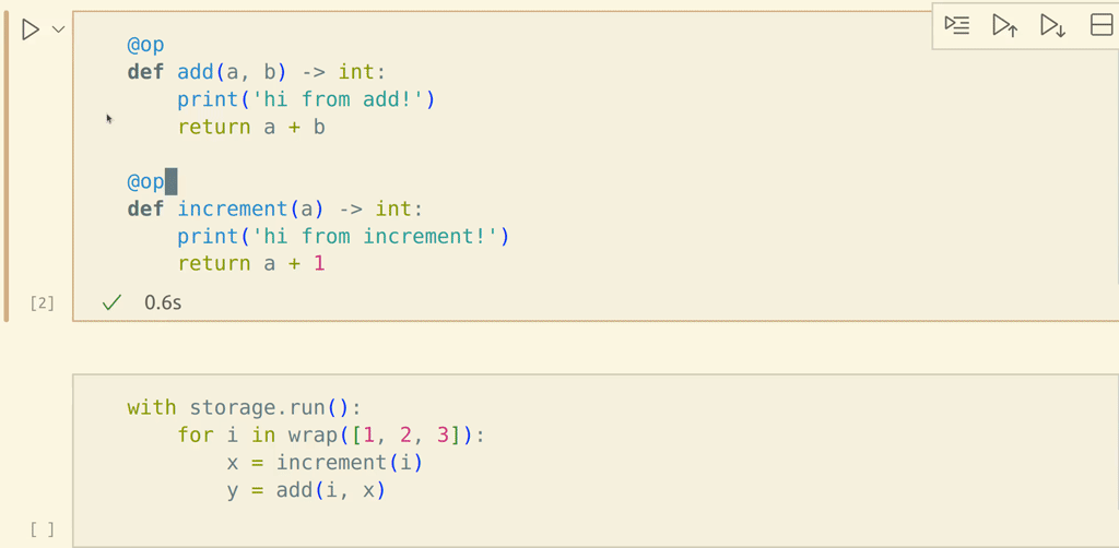
@op # core mandala decorator
def generate_data() -> Tuple[ndarray, ndarray]:
    ...

@op
def train_and_eval_tree(X, y, seed) -> Tuple[DecisionTreeClassifier, float]:
    ...
    
@op
def eval_forest(trees:List[DecisionTreeClassifier], X, y) -> float:
    # get majority vote accuracy
    ...

We can compose these functions in the obvious way to train a few trees and evaluate the resulting forest:

with storage.run(): # memoization context manager
    X, y = generate_data()
    trees = []
    for seed in range(10): # can't grow trees without seeds :)
        tree, acc = train_and_eval_tree(X, y, seed=seed)
        trees.append(tree)
    forest_acc = eval_forest(trees, X, y)

Note that we are passing the list trees of memoized values into another memoized function. This incurs no storage duplication, because each element of the list is stored separately, and trees behaves like a list of pointers to storage locations, rather than a monolithic blob. This is one example of how mandala’s memoization JustWorks™ with Python’s collections.

This compatibility lets you write algorithms that naturally operate on collections of objects (which do come up in practice, e.g. aggregators, model ensembling, clustering, chunking, …) in the most straightforward way, while still having intermediate results cached (and even declaratively queriable). The video below shows this in action by incrementally evolving the workflow above with new logic and parameters:

The video above illustrates

• memoization as imperative query interface: you can get to any of the computed quantities just by retracing the memoized code, or parts of it, again.
• laziness: when run against a persistent storage, mandala only reads from disk when a value is needed for a new computation
• control flow: laziness is designed to do the least work compatible with control flow - even though initially acc is a lazy reference, when the if acc > 0.8: statement is reached, this causes a read from the storage. This applies more generally to collections: a lazy reference to a collection has no elements, but e.g. iterating over it automatically loads (lazy) references to its elements.

Hierarchical memoization and (more) incremental computing

There’s still a major scalability problem - what if we had a workflow involving not tens but thousands or even millions of function calls? Stepping through each memoized call to get to a single final result (like we do with calls to train_and_eval_tree here) - even with laziness - could take a long time.

The solution is simple: memoize large subprograms like that end-to-end by abstracting them as a single (parametrized) memoized function. After all, every time there is a large number of calls happening, they share some repetitive structure that can be abstracted away. This way you can take “shortcuts” in the memoization graph:

The @superop decorator you see in the video is needed to indicate that a memoized function is itself a composition of memoized functions. A few of the nice things enabled by this:

• shortcutting via memoization: the first time when you run the refactored workflow, execution goes inside the body of train_forest and loops over all the memoized calls to train_and_eval_tree, but the second time it has already memoized the call to train_forest end-to-end and jumps right to the return value. That’s why the second run is faster!
• natively incremental computing: calling train_forest with a higher value of n_trees does not do all its work from scratch: since it internally uses memoized functions, it is able to (lazily) skip over the memoized calls and do only the new work.

Pattern-matching queries

Using memoization as a query interface relies on you knowing the “initial conditions” from which to start stepping through the trail of memoized calls - but this is not always a good fit. As a complement to this imperative interface, you also have a declarative query interface over the entire storage. To illustrate, consider where we might have left things with our random forest example:

In [23]: with storage.run():
   ...:     X, y = generate_data()
   ...:     for n_trees in (5, 10, ):
   ...:         trees = train_forest(X, y, n_trees)
   ...:         forest_acc = eval_forest(trees, X, y)

If this project went on for a while, you may not remember all the values of n_trees you ran this with. Fortunately, this code contains the repeated relationship between X, y, n_trees, trees, forest_acc you care about. In fact, the values of these local variables after this code executes are in exactly this relationship. Since every @op-decorated call links its inputs and outputs behind the scenes, you can inspect the qualitative history of forest_acc in this computation as a graph by calling storage.draw_graph(forest_acc):

This data makes it possible to directly point to the variable forest_acc and issue a query for all values in the storage that have the same qualitative computational history:

In [42]: storage.similar(forest_acc, context=True)
Pattern-matching to the following computational graph (all constraints apply):
    a0 = Q() # input to computation; can match anything
    X, y = generate_data()
    trees = train_forest(X=X, y=y, n_trees=a0)
    forest_acc = eval_forest(trees=trees, X=X, y=y)
    result = storage.df(a0, y, X, trees, forest_acc)
Out[42]:
   a0  y           X                            trees  forest_acc
2   5  [0, 1, ...  [[0.0, 0.0, ...  [DecisionTreeC...        0.96
3  10  [0, 1, ...  [[0.0, 0.0, ...  [DecisionTreeC...        0.99
0  15  [0, 1, ...  [[0.0, 0.0, ...  [DecisionTreeC...        0.99
1  20  [0, 1, ...  [[0.0, 0.0, ...  [DecisionTreeC...        0.99

The context=True option includes the values forest_acc depends on in the table. In particular, this reveals all the values of n_trees this workflow was ran with, and the intermediate results along the way.

Finally, you have an explicit counterpart to this implicit query interface: if you copy-paste the code for the computational graph above into a with storage.query(): block, result will be the same table as above.

What just happened? 🤯

Behind the scenes, the computational graph that forest_acc is derived from gets compiled to a SQL query over memoization tables. In the returned table, each row is a matching of values to the variables that satisfies all the computational relationships in the graph. This is the classical database concept of conjunctive queries.

And here’s (simplified) SQL code the pattern-matching query compiles to, where you should think of __objs__ as a table of all the Python objects in the storage:

SELECT a0, y, X, trees, forest_acc
FROM 
    __objs__.obj as a0, __objs__.obj as X, __objs__.obj as y,
    __objs__.obj as trees, __objs__.obj as forest_acc, ...
WHERE
    generate_data.output_0 = X and generate_data.output_1 = y and
    train_forest.X = X and train_forest.y = y and 
    train_forest.a0 = a0 and train_forest.output_0 = trees and
    eval_forest.trees = trees and eval_forest.X = X and eval_forest.y = y and
    eval_forest.output_0 = forest_acc

Pattern-matching with collections: the color refinement projection

You can propagate more complex relationships through the declarative interface, such as ones between a collection and its elements. This allows you to query programs that combine multiple objects in a single result (e.g., data aggregation, model ensembling, processing data in chunks, …) and/or generate a variable number of objects (e.g., clustering, …).

To illustrate, suppose that just for fun we disrupt the nice flow of our program by slicing into the list of trees to evaluate only on the first half:

with storage.run():
    X, y = generate_data()
    for n_trees in wrap((10, 15, 20)):
        trees = train_forest(X, y, n_trees)
        forest_acc = eval_forest(trees[:n_trees // 2], X, y)

If you look at how forest_acc is computed now, you get a substantially larger graph:

The problem is that there are now six (apparently, for n_trees=20, 12 or 13 trees survived the filtering!) chains of “get an element from trees, put it in a new list” computations in this graph that are redundant (they look exactly the same) and at the same time tie the graph to a particular value of n_trees. This will make the query both slow and too specific for our needs.

There is a principled solution to eliminate such repetition from any computational graph: a modified color refinement algorithm. There’s too many details for the scope of this blog post, but the overall intuition is that you can project¹ any computational graph to a smaller graph where there are no two vertices that “look the same” in the context of the entire computation². Here is what you get when you run storage.draw_graph(forest_acc, project=True):

And here is the code for this graph that you get using storage.print_graph(forest_acc, project=True):

idx0 = Q() # index into list
idx1 = Q() # index into list
X, y = generate_data()
n_trees = Q() # input to computation; can match anything
trees = train_forest(X=X, y=y, n_trees=n_trees)
a0 = trees[idx1] # a0 will match any element of a match for trees at index matching idx1
a1 = ListQ(elts=[a0], idxs=[idx0]) # a1 will match any list containing a match for a0 at index idx0
forest_acc = eval_forest(trees=a1, X=X, y=y)

Note how the two indices idx0, idx1 are different variables. This means that the result of this query will be larger than it intuitively needs to be, because there will be matches for one index in trees and another index in trees[:n_trees//2]. You can restrict it further by making idx0, idx1 the same variable.

Per-call versioning and dependency tracking

So far, we’ve treated memoized functions as unchanging, but that’s quite unrealistic. One of the thorniest problems of data management is maintaining a clear relationship between code and data in the face of changes in the internal logic of a project’s building blocks:

• if you ignore a change in logic, you generally end up with a mixture of results that look homogeneous to the system, but differ in the way they were generated. This makes comparisons between them more or less meaningless.
• if every change is automatically marked as a change in logic (looking at you, git), executions of semantically equivalent code will be confusingly scattered across versions. This makes comparisons between them difficult to program, and deters users from code quality improvements.

An automatic and universal solution to this problem is fundamentally impossible. What mandala offers instead is:

• per-call dependency tracking: automatically track the functions and global variables accessed by each memoized call, and alert you to changes in them, so you can (carefully) choose whether a change to a dependency requires recomputation of dependent calls
• content-addressable versions: use the current state of each dependency in your codebase to automatically determine the currently compatible versions of each memoized function to use in computation and queries. In particular, this means that:
  • you can go “back in time” and access the storage relative to an earlier state of the code (or even branch away in a new direction like in git) by just restoring this state
  • the code is the truth: when in doubt about the meaning of a result, you can just look at the current code.

Warmup: adding an argument backward-compatibly

A very common type of change in practice is to have a function you’ve run a few times, and then get an idea for how it could do its work differently (e.g. use a new algorithm, or vary a previously hardcoded constant). Importantly, you want to keep the old results around, but also somehow distinguish them from the new ones.

In mandala, you can do this by adding an argument with a default value, and it JustWorks™. A column is added to the function’s memoization table, with the default value applied retroactively to past calls. All the memoized calls without the new argument are still memoized. When doing this with a versioned storage, you’ll be shown a diff and should mark the change as not requiring recomputation of dependents:

Marking changes as breaking and traveling back in time

When you discover a bug affecting results, or just want to change how a function works and recompute everything that depends on it, you mark the change as requiring recomputation in the diff dialog. This will essentially tell the storage that this function now “means something else” (under the hood, it has a different semantic id from the previous version).

If you want to revisit the old results, restore the code to the old state; this will cause the storage to interpret the function according to its previous meaning in both computation and queries. You can examine the “shallow” versions of a dependency (i.e. the revisions of its own source code) with storage.sources(f), and the “deep” versions (which include sets of dependencies as seen by calls to this function) with storage.versions(f):

Conclusion

This was a rather brisk walk through mandala, but it hopefully gave you an idea of its general spirit and the particular ways in which it simplifies computational data management. Some features that were not mentioned here, but are currently in the works:

• batch execution: separate data management and execution concerns in cases when it’s more efficient to run function calls in batches, such as inference on large machine learning models. Code inside a with storage.batch() context is executed by a custom (batched) executor that you can implement, yet each call is individually memoized and queriable.
• parallelization: since mandala is function-based, it’s a great fit for function-based parallelization frameworks like dask.
• deletion interfaces: an imperative/declarative deletion interface, analogous to the imperative/declarative query interfaces. Just change with storage.run() to with storage.delete().

We invite you to try mandala for your own projects and welcome contributions to help improve its performance and capabilities!

Acknowledgements

Thanks to Stefan Krastanov, Melody Guan and Ben Kuhn for providing feedback on drafts of this post.